The tensor product: why 10 qubits means 1024 numbers

You hear it constantly. Quantum computers are exponentially powerful. The state space doubles with every qubit. It is the line that makes quantum sound like magic and makes you feel like you are missing something. You are not missing much. The exponential comes from one operation, the tensor product, and it is far simpler than the word suggests. Combine two qubits and you get four numbers. Here is exactly how, by hand.

Start with the counting

One qubit is two numbers. The amplitude on |0⟩ and the amplitude on |1⟩, the pair from the very first posts. Two amplitudes, and squaring their lengths gives the probabilities.

Two qubits is four numbers. The possible outcomes are 00, 01, 10, and 11, and there is an amplitude on each, so four amplitudes describe the pair. Three qubits is eight, the outcomes running 000 through 111. You can already feel the pattern, and the operation that builds the bigger list out of the smaller ones is the tensor product.

How to actually compute it

The tensor product takes two vectors and builds a longer one by a simple, mechanical rule: multiply each entry of the first by the whole of the second, and stack the results. For two qubits, [a, b] tensored with [c, d] gives [ac, ad, bc, bd]. NumPy spells the tensor product kron, for Kronecker product, which is the same thing.

import numpy as np
print(np.kron([1, 0], [1, 0]))   # [1 0 0 0]   ->  |00>
print(np.kron([1, 0], [0, 1]))   # [0 1 0 0]   ->  |01>

Run it. The state |0⟩ tensored with |0⟩ is [1, 0, 0, 0], a vector of length four with all its weight on the first slot, which is the |00⟩ outcome. |0⟩ tensored with |1⟩ puts the weight on the second slot, |01⟩. The four slots of the combined vector are exactly the four outcomes 00, 01, 10, 11, in order. Try it with a superposition and nothing changes about the mechanism.

plus = np.array([1, 1]) / np.sqrt(2)        # |+>
print(np.round(np.kron(plus, [1, 0]), 3))   # [0.707 0 0.707 0]

Run it. |+⟩ tensored with |0⟩ spreads its weight across the 00 and 10 slots, which says the first qubit is undecided and the second is firmly 0, exactly what you put in. The tensor product is just bookkeeping for combining independent qubits into one description, and you can do it on paper for two qubits without strain.

Three qubits, and which slot is which

The operation chains. For three qubits you tensor three vectors, left to right, and the result has eight slots.

k = np.kron(np.kron([1, 0], [1, 0]), [1, 0])
print(k, "length", len(k))   # [1 0 0 0 0 0 0 0]  length 8

Run it. Three copies of |0⟩ tensor to |000⟩, a length eight vector with all its weight on the first slot. And here is the indexing rule that makes a long amplitude vector readable, because it confused me at first. The slots are just the outcomes counted in binary. Slot 0 is 000, slot 1 is 001, slot 2 is 010, and so on up to slot 7, which is 111. So the position in the vector is the binary number of the outcome it represents. Once you see that, a vector of sixteen amplitudes for four qubits stops being an intimidating wall of numbers and becomes an ordered list: slot five is outcome 0101, and the length of its amplitude, squared, is the probability of measuring 0101. The tensor product lays the outcomes out in plain binary order, every time, which is the thing that lets you actually read these vectors instead of drowning in them.

The doubling, and where the reputation comes from

Now watch the counts as you add qubits, because this is the whole point.

for n in [1, 2, 3, 10, 20]:
    print(f"{n} qubits -> {2**n} amplitudes")

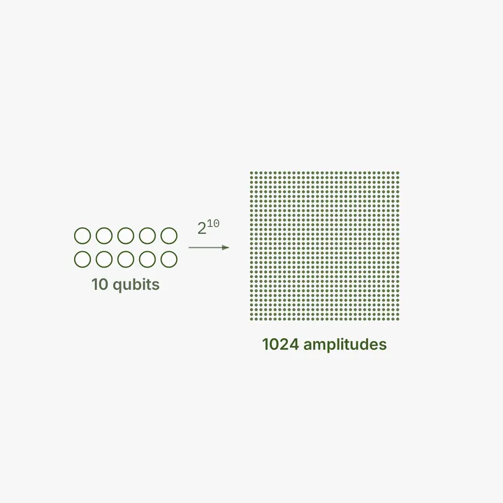
Run it. One qubit, two amplitudes. Two qubits, four. Three, eight. Ten qubits, one thousand and twenty four numbers. Twenty qubits, over a million. Each qubit you add doubles the length of the vector, because tensoring with one more two slot qubit doubles the slots. n qubits is described by 2 to the power n complex numbers. That is the exponential everyone keeps pointing at, and it is not a vague slogan, it is just this doubling, compounding.

The numbers get absurd fast. At fifty qubits you are past a quadrillion amplitudes. At three hundred qubits, the count of amplitudes exceeds the number of atoms in the observable universe. A modest pile of qubits describes a state living in a space so large you could never write it down. That enormous space, all of it evolving together when you apply a gate, is the arena quantum computing plays in. That is where the power is supposed to come from.

The same exponential is also the wall

Here is the part the hype usually skips, and it is the most useful thing in this post. The exponential that makes quantum powerful is the exact same exponential that makes quantum hard to fake.

To simulate n qubits on an ordinary computer, you have to store those 2 to the n amplitudes in memory and update them. Thirty qubits is already a billion numbers, heavy but doable on a big machine. Around fifty qubits you blow past what any classical computer on Earth can hold, because each extra qubit doubles the memory and the doubling wins, always and quickly. This is why you cannot just simulate a large quantum computer on a laptop, or a supercomputer, or all the supercomputers together. The state does not fit. And it is the deepest reason real quantum hardware matters: a physical qubit holds its share of that exponential state for free, as a matter of physics, where a classical simulation has to pay for every amplitude in memory it does not have. The doubling is the promise and the wall at once. Respect it from both sides.

Put real numbers on it to feel the wall. Each amplitude is a complex number, call it sixteen bytes. Fifty qubits is 2 to the fifty amplitudes, which is over a quadrillion, times sixteen bytes, which lands around sixteen petabytes of memory just to hold the state for an instant, before you have done a single operation on it. Sixty qubits is another thousandfold on top of that. There is no cluster you can rent that makes this go away, because the problem is not engineering, it is the exponent, and you cannot out build an exponent. Every qubit added does not make the simulation a bit harder. It doubles it. That cliff, sitting somewhere around fifty qubits, is precisely the line past which no honest state vector simulation can follow. Specialised methods can still reach past it on circuits with enough structure to exploit, sometimes exactly, by never storing the whole vector at all. None of them repeal the general case, and none of them move the memory wall.

Gates scale by tensoring too

One loose end, because it ties back to the gates post. When you have several qubits and you apply a gate to just one of them, that gate is also a tensor product. A Hadamard on the left qubit of a two qubit system is really H tensored with the identity on the right one, because the untouched qubit gets the do nothing matrix. The result is a bigger matrix that acts on the whole combined vector.

H = np.array([[1, 1], [1, -1]]) / np.sqrt(2)
I = np.eye(2)
print(np.kron(H, I).shape)   # (4, 4)

Run it. H tensored with I is a four by four matrix, the right size to multiply the four slot state of two qubits. So the entire picture from the gates post, apply a gate by multiplying a matrix, scales up cleanly: act on one qubit by tensoring its gate with identities on the rest, and the mechanism is unchanged, just larger. Everything is still matrix times vector. The vectors and matrices simply grow with the tensor product.

And tensoring two real gates together pays off immediately. Put a Hadamard on each of two qubits, both starting in |0⟩, and watch what comes out.

HH = np.kron(H, H)
print(np.round(HH @ np.array([1, 0, 0, 0]), 3))   # [0.5 0.5 0.5 0.5]

Run it. H tensored with H, applied to |00⟩, gives [0.5, 0.5, 0.5, 0.5], equal amplitude on all four outcomes. Two Hadamards just put two qubits into superposition at once, and the tensor product turned that into a single state spread evenly over 00, 01, 10, 11. Scale this up and it is the move behind a huge amount of quantum computing: a Hadamard on every one of n qubits produces an equal superposition over all 2 to the n outcomes in one layer of gates. That is how an algorithm gets the entire input space into play simultaneously, and it is nothing but the tensor product doing its doubling, gate side this time instead of state side.

The entanglement connection

This is also where the last post and this one meet. The tensor product builds the big combined space by gluing independent qubits together. A state that was built that way, by tensoring separate qubits, is a product state, and it always factors back into its parts. But the combined space, all 2 to the n slots of it, contains far more vectors than just the ones you can build by tensoring. Most of the vectors in there cannot be factored into separate qubit states at all. Those are the entangled states. The Bell state from last time is one of them, a four slot vector that no tensor product of two qubits can produce. So the tensor product builds the room, and entanglement is everything in the room that cannot be taken back apart. The two ideas are two halves of the same picture.

Order matters: which qubit goes where

One practical wrinkle, because it connects to a warning from earlier posts. The tensor product is not symmetric. |0⟩ tensored with |1⟩ is [0, 1, 0, 0], the outcome 01, while |1⟩ tensored with |0⟩ is [0, 0, 1, 0], the outcome 10. Same two qubits, opposite order, different state. So when you combine qubits, you have to keep track of which one is on the left and which on the right, because the order decides which slot each outcome lands in.

This is the same little endian issue that bit me in the Python and gates posts. Qiskit orders its qubits in the reverse of the textbook convention, qubit 0 on the right of the string, so a state your hand calculation labels one way may be labelled the mirror way by the library. Neither is wrong, they are conventions, but if you tensor in one order and the tool reports in the other, you will stare at a vector that looks scrambled until you remember the order is flipped. The fix is just awareness: pick a convention, know which one your tool uses, and the slots line up. The tensor product is mechanical, but it is not order blind, and quietly assuming it is costs you an afternoon of confusion you do not need to have.

The difference from classical bits, which is the whole point

There is a confusion worth heading off, because it tripped me and it hides the real source of the power. You might object that classical bits also have 2 to the n possible states. Eight bits can represent any of two hundred and fifty six values, ten bits a thousand and twenty four, the same exponential. So what is special?

The difference is everything. With n classical bits, there are 2 to the n possible states, but at any moment you hold exactly one of them. Ten bits store one number out of a thousand, the one they happen to be set to. The exponential is just the size of the menu, and you are only ever eating one dish. With n qubits, the state is not one of the 2 to the n possibilities, it is an amplitude on all of them at once, the full vector live and present together. Ten qubits do not hold one of a thousand numbers. They hold a thousand and twenty four amplitudes simultaneously, every outcome carrying its own complex weight, all of them there at the same time.

That is the gap classical intuition misses. The classical machine has an exponential number of possible configurations and occupies one. The quantum machine occupies an object that has an exponential number of parts. When you apply a gate, you act on the entire vector in one go, nudging all 2 to the n amplitudes together, which is the closest honest description of where the much abused phrase massive parallelism comes from. The catch, and there is always a catch, is that measurement still hands you back just one outcome, so the art of a quantum algorithm is steering that giant vector with interference so that the outcome you want is the one likely to appear. The exponential state is real and present. Reading it out is the part you have to be clever about.

A quick test before you move on

Close this and answer in your own words.

How many complex numbers describe the state of eight qubits? If you did not immediately think two to the eighth, which is two hundred and fifty six, the doubling has not become automatic yet, so go back to the counting.

What is the actual rule for tensoring [a, b] with [c, d]? If you cannot produce [ac, ad, bc, bd], reread the how to compute it section, because that mechanical step is the whole operation.

And why can you not store the state of a fifty qubit quantum computer on a classical machine? If your answer does not mention that the memory doubles per qubit, the section on the wall did not land.

Where I am learning it

Free. For the linear algebra underneath, 3Blue1Brown is again the clearest on what these vectors and matrices actually are, and any introduction to the Kronecker product fills in the mechanics. The exponential blowup is one of those things that is obvious once you compute it and abstract until you do, so the most useful exercise was the tiny loop above, watching the amplitude count double and double until the numbers stopped meaning anything. As always, I keep these as NumPy I can rerun, because a doubling I have only read about does not land like a doubling I have watched run off the end of what any machine could hold.

One humble operation

For a long time the exponential power of quantum sat in my head as a kind of slogan, something true that I could repeat without really feeling. It turned out to rest on one of the plainest operations in the whole subject, a bookkeeping rule for combining vectors that you can do by hand for two qubits in a few seconds.

The tensor product is not where the difficulty lives. The difficulty lives in what it implies, the relentless doubling that builds a state space too big to write down, powering the machine on one side and defeating every attempt to simulate it on the other. The operation is humble. The consequence is the entire reason the field exists. Worth knowing which is which.