Quantum gates are just matrices you can run by hand

The word gate tripped me up for longer than I want to admit. It sounds like hardware. A physical component, a little door the qubit passes through, something happening at the level of atoms and lasers that I would need a physics degree to follow. So I treated quantum gates as magic for a while, things that did mysterious quantum stuff by means I was not equipped to question.

Then the math notebook and the Python post collided in my head and the whole thing collapsed into something almost embarrassingly simple. A qubit is a vector. A gate is a matrix. Applying a gate is multiplying the matrix by the vector. That is the entire mechanism. Not a metaphor, not an approximation. Literally that. Here are the gates that matter, what each one does, and the two laws they all obey, all of it runnable by hand.

Apply a gate, by multiplying

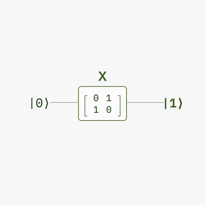
Start with the simplest possible case so the claim is concrete. The X gate is the quantum NOT. Here it is as a matrix, applied to the state |0⟩, which is the vector [1, 0]:

import numpy as np
X = np.array([[0, 1], [1, 0]])
ket0 = np.array([1, 0])
print(X @ ket0)     # [0 1]  ->  |1>

Run it. The X gate turned |0⟩ into |1⟩, a bit flip, and the act of applying it was a single matrix multiply, the @ from the Python post. That is what a gate does, every time, no exception. You take the matrix, you multiply it by the state vector, and the result is the new state. Everything below is just a catalogue of which matrices are worth knowing and what each one does to the vector. Once you have this picture, gate stops being a mysterious noun and becomes a thing you can compute on paper.

The single qubit gates worth knowing

There are a handful you will see constantly. Here is each one as a matrix and, more usefully, as a thing it does.

X, the NOT. Swaps |0⟩ and |1⟩. The quantum bit flip, and the most familiar one because it has a classical twin.

Z, the phase flip. Leaves |0⟩ completely alone and flips the sign of |1⟩.

Z = np.array([[1, 0], [0, -1]])
ket1 = np.array([0, 1])
print(Z @ ket1)     # [0 -1]  ->  -|1>

Run it. |1⟩ became −|1⟩. Nothing about the probability changed, since the modulus is the same, but the sign did, and that sign is a phase. Hold that thought. It is the seed of an entire later post.

H, the Hadamard. The workhorse of the whole field. It turns the definite states into superpositions and back. H on |0⟩ gives the equal superposition |+⟩, and because it is its own inverse, H on |+⟩ gives you |0⟩ right back. Almost every circuit you will ever read opens with a Hadamard somewhere, because it is how you get a qubit off the fence and into superposition in the first place.

s = 1/np.sqrt(2)
H = s * np.array([[1, 1], [1, -1]])
print(np.round(H @ ket0, 3))     # [0.707 0.707]  ->  |+>

Run it. The same matrix multiply as the X gate, just a different matrix, and out comes the superposition. There is nothing special about how you apply it. Every gate is the same act.

Y, the third Pauli. Effectively X and Z at once, with a factor of i mixed in. You will meet it constantly as a name, less often as something you apply by hand early on, so file it next to X and Z and move on.

S and T, the phase gates. These rotate the phase of the |1⟩ part without touching its probability. S adds a quarter turn, T adds an eighth turn. Remember from the complex numbers post that multiplying by i is a quarter turn on the circle. That is exactly what S does to the |1⟩ amplitude.

S = np.array([[1, 0], [0, 1j]])
print(S @ ket1)     # [0 i]  ->  i|1>,  a quarter turn of phase

Run it. S sent |1⟩ to i times |1⟩, a ninety degree phase rotation, the quarter turn you already understand. And T is the half of S, in the sense that applying T twice equals S, which is a nice thing to verify yourself in a moment.

Two laws every gate obeys, and why they matter

Not every matrix is a legal gate. They all satisfy two conditions, and both conditions mean something physical.

Every gate is unitary. Formally, the dagger of the matrix times the matrix equals the identity, U† U = I, using the conjugate transpose from the Python post. What it means in plain terms is that a gate preserves length. A valid quantum state is a vector of length one, because its squared amplitudes are probabilities and probabilities sum to one. A gate has to keep that true. It can rotate the state, point it anywhere, but it can never stretch or shrink it, because a state of the wrong length would have probabilities that do not add up to one, which is nonsense. Unitary is just the mathematical way of saying this gate respects the rules of probability. And you can check it, the same way you check anything, with an assertion.

I = np.eye(2)
H = (1/np.sqrt(2)) * np.array([[1, 1], [1, -1]])
assert np.allclose(H.conj().T @ H, I), "H is not unitary"
print("H is unitary")

Run it. It passes in silence, the way a true assertion does.

Every gate is reversible. This one is quietly profound. Because gates are unitary, every single one has an inverse, which means every quantum operation can be undone. There is always a gate that takes you exactly back. Some gates are even their own inverse, Hadamard most famously: apply it twice and you are precisely where you started.

assert np.allclose(H @ H, I)        # H undoes itself
print("H applied twice is the identity")

Run it. This is a deep break from classical computing. An ordinary AND gate takes two bits in and gives one bit out, and from that one output you cannot recover the two inputs. Information is destroyed. Classical logic throws things away constantly. Quantum gates never can. Every operation is a reversible rotation, nothing is lost, and that single fact shapes an enormous amount of how quantum computing actually works. It is also worth a verification of its own. Remember the claim that two T gates make an S?

T = np.array([[1, 0], [0, np.exp(1j*np.pi/4)]])
assert np.allclose(T @ T, S)        # T is the 'square root' of S
print("T squared equals S")

Run it. T applied twice is exactly S, the eighth turn done twice making a quarter turn, which is just addition of angles dressed up as matrix multiplication.

Stacking gates is just multiplying matrices

Here is the step that turns single gates into a whole circuit, and it is short. A circuit is a sequence of gates applied one after another. Applying gate A and then gate B to a state is just B times the result of A times the state, which by the way matrix multiplication works equals the single matrix B times A, applied once. So an entire circuit collapses into one matrix, the product of all its gates, and running the circuit is multiplying that one matrix against your starting state.

Two things fall out of this, both worth holding. The first is order. You multiply right to left, in the reverse of the order you apply the gates, because the gate you apply first sits closest to the state. And order matters, because matrices do not generally commute. X then Z is not the same as Z then X.

print(np.allclose(X @ Z, Z @ X))   # False, order matters

Run it. They disagree, which is the mathematical version of saying the sequence of operations changes the result, exactly as you would expect from anything done in steps. The second thing that falls out is the prettiest small fact in the early going. A Hadamard, then a Z, then a Hadamard, equals an X. Three gates, multiplied together, collapse to a single different gate.

print(np.allclose(H @ Z @ H, X))   # True

Run it. H Z H is X, exactly. A phase flip wrapped in two Hadamards becomes a bit flip. This is not a coincidence, it is the rotation picture coming next, but even before that picture it is a concrete, checkable demonstration that gates compose by multiplication and that the composition can be something genuinely new. A whole circuit is one matrix you could, in principle, work out by hand. That is the entire idea of a circuit, hiding inside one line of NumPy.

Gates are rotations

Here is the picture that ties it all together. A single qubit's state can be drawn as a point on the surface of a sphere, called the Bloch sphere. |0⟩ at the north pole, |1⟩ at the south, the superpositions around the equator. You do not need the full machinery of it to take the one useful idea away, which is this: every single qubit gate is a rotation of that point. X, Y, and Z are half turns about three different axes. H is a particular rotation that swaps poles for equator. And there is a whole continuous family, written RX, RY, and RZ, that rotate the state by any angle you like about each axis.

def RX(theta):
    c, s = np.cos(theta/2), np.sin(theta/2)
    return np.array([[c, -1j*s], [-1j*s, c]])

print(np.allclose(RX(np.pi), -1j*X))   # True

Run it. A rotation of half a turn about the X axis is the X gate itself, give or take an overall phase factor. This is why the complex numbers post mattered so much. Multiplication by complex numbers is rotation, gates are rotations, and the two facts are the same fact seen from two angles. Once gates became rotations in my head, the discrete named gates and the continuous angle gates stopped being two separate topics and became one. Fixed gates are just rotations by special, useful angles.

Two qubit gates, and the one that matters most

Everything so far acts on a single qubit. The interesting things happen when gates act on two at once, and the one to know is CNOT, controlled NOT. It is a four by four matrix, because two qubits live in a four dimensional space, and what it does is conditional. It flips the second qubit, the target, but only if the first qubit, the control, is 1. If the control is 0, it does nothing.

CNOT = np.array([[1, 0, 0, 0],
                 [0, 1, 0, 0],
                 [0, 0, 0, 1],
                 [0, 0, 1, 0]])
print(CNOT @ np.array([0, 0, 1, 0]))   # |10> -> |11>

Run it. The state |10⟩, control 1 and target 0, came out as |11⟩, target flipped. CNOT is the gate that lets qubits affect each other, and it is the doorway to entanglement, which deserves and will get its own post. For now, just add it to the catalogue. A bigger matrix, doing a conditional flip, multiplied against a bigger vector. Same mechanism as everything else.

In Qiskit, versus by hand

In practice you will not multiply these matrices yourself. You will write qc.h(0) and qc.cx(0, 1), and Qiskit assembles the circuit for you, exactly as the Python post described, methods called on a circuit object. But the point of doing it by hand even once is that you can, and that you can check the library against your own arithmetic when something looks off. Qiskit will even hand you a circuit's matrix if you ask for it, through an Operator, so you can compare it to the one you built.

One honest warning, the same one from the Python post. Qiskit numbers its qubits in the reverse of the textbook convention, qubit 0 on the right, little endian. So a CNOT matrix you pull out of Qiskit may not look identical to the one above, not because either is wrong, but because the qubit order is flipped. Knowing that the ordering convention exists saves you the exact evening I would otherwise have lost to it.

A few gates are all you need

One more fact worth carrying, because it surprised me and it changes how you see the whole catalogue. You do not need a separate exotic gate for every operation you might want. A small handful of gates is enough to build, to any precision you like, any circuit at all. A common universal set is the Hadamard, the T, and the CNOT. With just those three, composed in the right order and number, you can approximate any quantum computation there is.

If that rings a bell, it should. Classical computing has the same property: every logic circuit you have ever used can be built from NAND gates alone. Universality is not a quantum quirk, it is a deep and reassuring fact about computation in general. A tiny, fixed alphabet, combined cleverly, expresses everything. It means hardware builders can pour their effort into making a few gates extremely well rather than chasing an infinite zoo, and it means that when you learn this short list, you are not learning a sample of the gates. You are learning, in a real sense, all of them, because the rest are just these few stacked up. The catalogue is not endless. It only looked that way from the outside.

A quick test before you move on

Close this and answer in your own words.

What does applying a gate to a state actually do, mechanically? If your answer is not multiplies a matrix by a vector, the whole post did not land, so go back to the top.

Why must every gate be unitary, in terms of probability? And what does unitary buy you that classical logic does not have? If reversible and nothing is destroyed are not in your answer, reread the two laws.

And what do the S and T gates do to a state, and how does that connect to multiplying by i? If you cannot tie a phase gate to a quarter turn, that is your gap, and it is the one that pays off most later.

Where I am learning it

Free and, for this, visual is everything. 3Blue1Brown's linear algebra series is the single best thing I have watched for seeing a matrix as a transformation rather than a grid of numbers, which is the exact shift that makes gates click. MIT's 18.06 goes deeper if you want the full foundation. And my own notebook of gates as NumPy arrays, the one from the Python post, is where I actually check all of this, because a gate I have only read about is not a gate I trust until I have multiplied it against a state myself and watched the vector move.

The magic was just a matrix

Gate was the word that kept quantum feeling like a closed door. It sounded like hardware, like physics I had no claim to. It turned out to be a matrix, and applying it turned out to be the matrix multiply I already knew from the Python post, and the whole exotic vocabulary resolved into linear algebra I could do on paper.

The hardware really is exotic. Building a physical qubit and holding it steady is genuinely the work of brilliant people with cryogenic fridges. But the gates, the part I was actually afraid of, the part I have to reason about to write a circuit, are not exotic at all. They are matrices. And I already know how to multiply a matrix by a vector. So do you.