Measurement is not magic: the Born rule by hand
Why a quantum result is a probability: amplitude squared, worked on paper and checked in NumPy, one basis at a time.

Earlier in this series I made a case that a qubit is not a coin under a cup. It is a vector with two amplitudes, turning under exact rotations, undecided about nothing, right up until you look. Which leaves the obvious question hanging. Fine. So what exactly happens when you look?
That is measurement, and it is the step everyone treats as the mystical one. The wave function collapses. The universe decides. Cue the dramatic music. I needed something I could actually use, so I went looking for the mechanism, and it turned out to be one short formula. Once I could run it by hand, measurement stopped being the magic step and became, in aggregate, the most predictable thing in the whole machine.
Here is that formula, and everything that falls out of it.
The whole rule, in one line
This is the Born rule, and it is the most important equation in quantum computing. Every histogram you will ever stare at is this, and nothing but this.
P(k) = |⟨k|ψ⟩|²
In words. The probability of getting outcome k when you measure the state |ψ⟩ is the squared size of the overlap between k and ψ. That overlap, the ⟨k|ψ⟩ part, is a single number called the inner product. Take its magnitude, square it, and you have your probability.
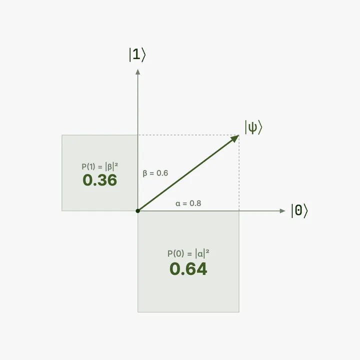
You have already met the easy version of this. When I wrote that a qubit α|0⟩ + β|1⟩ gives 0 with probability |α|² and 1 with probability |β|², that was the Born rule in its simplest case, where the thing you measure is one of the basis states. The general formula above is the same idea with the training wheels off. It works for any measurement, not just the obvious one, and that generality is where measurement gets genuinely interesting.
So before anything else, I had to actually understand that ⟨k|ψ⟩ object.
The inner product is just overlap
The inner product takes two states and returns one number. You multiply them component by component and add up the results. The only twist is that the first one, the part written as a bra ⟨ |, gets conjugated, which for real numbers changes nothing and just gives you the ordinary dot product you already know.
What it means is the useful part. The inner product measures how much two states overlap. If it is zero, the states are orthogonal, completely distinct, perfectly distinguishable. If its size is one, they are the same state. Everything in between is partial overlap.
The two facts you lean on constantly:
⟨0|0⟩ = 1, a state fully overlaps with itself. ⟨0|1⟩ = 0, the states |0⟩ and |1⟩ are orthogonal, no overlap at all.
Let me do one that is not just 0 or 1, by hand, because it is worth seeing once. Take the overlap of |0⟩ with the superposition |+⟩ = (|0⟩ + |1⟩)/√2. Writing |0⟩ as the column [1, 0] and |+⟩ as [1/√2, 1/√2], the inner product multiplies matching entries and adds them: 1 times 1/√2, plus 0 times 1/√2, which is just 1/√2. Square that and you get one half. So the chance of measuring 0 from |+⟩ is one half, computed straight from the overlap. The same arithmetic in NumPy, as a check:
import numpy as np
s = 1/np.sqrt(2)
ket0 = np.array([1, 0]); plus = s*np.array([1, 1])
print(np.vdot(ket0, plus))        # 0.7071...  the overlap <0|+>
print(round(abs(np.vdot(ket0, plus))**2, 12)) # 0.5   the probability
Put that together with the Born rule and a clean sentence falls out, the one that finally made measurement make sense to me. |⟨k|ψ⟩|² is the probability of finding your state behaving like k when you measure. It is overlap, squared, turned into odds. Measurement asks how much does my state look like this outcome, and the answer, squared, is how often you get it.
Measurement depends on the question you ask
Here is the part that is genuinely deeper than amplitudes squared, and the part most explanations skip.
Take the equal superposition from earlier, the state |+⟩ = (|0⟩ + |1⟩)/√2. Measure it in the ordinary 0 and 1 basis. The overlaps are each 1/√2, so each probability is one half. Fifty fifty. Exactly the quantum coin everyone expects.
import numpy as np
s = 1/np.sqrt(2)

ket0  = np.array([1, 0])
ket1  = np.array([0, 1])
plus  = s * np.array([1,  1])   # |+>
minus = s * np.array([1, -1])   # |->

# np.vdot(a, b) conjugates a, so it is exactly <a|b>
print(round(abs(np.vdot(ket0, plus))**2, 12))   # 0.5   P(0)
print(round(abs(np.vdot(ket1, plus))**2, 12))   # 0.5   P(1)
Run it. Both come out to one half, as promised. So far, coin.
Now measure the very same state in a different basis, the plus and minus basis, the one built from |+⟩ and |−⟩. Nothing about the qubit changes. Only the question changes.
print(round(abs(np.vdot(plus,  plus))**2, 12))         # 1.0   P(+)
print(round(abs(np.vdot(minus, plus))**2, 12)) # 0.0   P(-)
Certain. In this basis the same state gives |+⟩ every single time, with zero chance of |−⟩. The fifty fifty was never a property of the qubit. It was a property of the question I happened to ask it.
This is what I meant earlier when I said a superposition is a definite state, not an uncertain one. |+⟩ is not unsure of itself. It is pointing in a perfectly definite direction. It only looks random when you insist on measuring it along the 0 and 1 axis, which is not the axis it is pointing along. Ask it the right question and it answers without hesitation. Measurement does not reveal a hidden value the qubit was secretly holding. It compares the qubit against whatever outcomes your chosen measurement offers, by overlap, and then rolls the dice the Born rule hands it.
How you actually measure in another basis
There is a catch I glossed over, and it is the part that connects measurement back to gates. Real hardware only knows how to measure in one basis, the ordinary 0 and 1 one. You do not get a dial for measuring in the plus and minus basis instead. So how do you ever ask a different question?
You move the question to the measurement, instead of the other way around. Before you measure, you apply a gate that rotates the basis you care about onto the 0 and 1 axis. Then you measure normally, and you relabel the outcomes. For the plus and minus basis, that rotating gate is the Hadamard.
import numpy as np
s = 1/np.sqrt(2)
H = s*np.array([[1, 1], [1, -1]])
plus = s*np.array([1, 1])

print(np.round(H @ plus, 12))   # [1. 0.]  ->  |0>, a certain result
Run it. The Hadamard turns |+⟩ into plain |0⟩, so now an ordinary measurement gives 0 every time, which you read as the |+⟩ outcome. That is exactly the certainty we computed with the inner product, arrived at a second way. Measuring |+⟩ in the plus and minus basis and applying a Hadamard then measuring in the normal basis are the same experiment.
This is why so many circuits end with a gate sitting right before the measurement. That last gate is not part of the computation. It is choosing which question you are about to ask the qubit. Once I saw that, the structure of real circuits clicked. The middle does the work, and the gate at the end picks the basis you read out in.
One measurement tells you almost nothing
A consequence that confused me until I sat with it. A single measurement is nearly useless.
Measure once and you get one outcome. A 0 or a 1. From that one bit you cannot recover the amplitudes, you cannot see the probabilities, you learn almost nothing about the state you prepared. The amplitudes are really there, but measurement does not report them. It samples from them, once, and hands you the single result it drew.
So you do the only thing you can. You run the whole thing again. And again. Thousands of times. Each run, called a shot, gives you one more sample, and as the samples pile up, their proportions close in on the true probabilities.
import numpy as np
rng = np.random.default_rng(0)

# 10000 measurements of |+> in the 0/1 basis: each is 0 or 1, fifty fifty
shots = rng.choice([0, 1], size=10000, p=[0.5, 0.5])
values, counts = np.unique(shots, return_counts=True)
print(dict(zip(values.tolist(), counts.tolist())))   # roughly {0: 5000, 1: 5000}
Run it. You get something close to five thousand of each, drifting closer to the true split the more shots you take. An exact five thousand split does happen, just rarely: the probability is about 0.8 percent, roughly one run in 125. This is exactly why a quantum result comes back as a dictionary of counts rather than a clean probability. The hardware cannot tell you the probability directly. It can only let you sample, so you sample a lot and read the proportions off the histogram. That counts dictionary you get from Qiskit is just this experiment, run on real qubits.
How many shots is enough is its own small art. The wobble around the true value shrinks slowly, roughly with the square root of the number of shots, which means to halve your uncertainty you need four times as many runs. A thousand shots pins a fifty fifty split down to a percent or two. Chasing a tiny difference between two outcomes can take far more. This is the quiet tax of a probabilistic machine. You are never reading an answer, you are estimating one, and a sharper estimate costs real time on the hardware. It is the same reason a poll of a few thousand people has a margin of error, and the same math sets it.
The expectation value, or the number you actually report
Often you do not even want the full distribution. You want one summary number, and there is a standard one. The expectation value is the long run average of the outcomes, each outcome weighted by how likely it is.
E[X] = the sum of each outcome times its probability
On a fair die, that is 1 through 6 each with probability one sixth, which averages to 3.5. The die never lands on 3.5. It is just where the average settles.
In quantum you do the same thing with a small convention. Label the outcome |0⟩ as +1 and the outcome |1⟩ as −1. The expectation value of that labelling is written ⟨Z⟩, and it tells you, in a single number, which way the qubit leans.
import numpy as np
ket0 = np.array([1, 0]); ket1 = np.array([0, 1])
s = 1/np.sqrt(2)

for name, state in [("|0>", ket0), ("|+>", s*np.array([1, 1])), ("|1>", ket1)]:
    p0 = abs(np.vdot(ket0, state))**2
    p1 = abs(np.vdot(ket1, state))**2
    print(name, "<Z> =", round((+1)*p0 + (-1)*p1, 12))
Run it. |0⟩ gives +1, a guaranteed up. |1⟩ gives −1, a guaranteed down. And |+⟩ gives exactly 0, perfectly balanced between the two, which is the number's way of saying fifty fifty. This is what Qiskit's estimator primitive computes for you, and it is what an enormous number of quantum algorithms actually read out at the end. Not a full histogram. One expectation value.
Worth doing the |+⟩ case by hand, since it is one line and it demystifies the symbol. For |+⟩ the two probabilities are each one half. So ⟨Z⟩ is (+1) times one half, plus (−1) times one half, which is one half minus one half, which is zero. The qubit leans neither way. A result of +1 would mean certainly 0, a result of −1 would mean certainly 1, and everything between is a lean in one direction. That single number captures the balance of the whole distribution.
This matters because a whole family of important algorithms is built to be read this way. The ones people are actually trying to run on today's noisy hardware, the chemistry and optimisation routines with names like VQE, work by adjusting a circuit to push an expectation value as low as it will go. They never ask for the full histogram. They ask for one number, over and over, and steer by it. So the humble weighted average is not a side note. For a large slice of near term quantum, it is the entire output.
And then the state is gone
The last piece, and the one with real consequences for how you write circuits.
Measurement is not a peek. It is destructive. The moment you measure |+⟩ and get a 0, the qubit is now |0⟩, full stop. The superposition you carefully built is spent. Measure it again and you will get 0 again, because there is no superposition left to sample, just a plain 0 sitting there.
This is why you cannot prepare one state and measure it a thousand times to gather your statistics. The first measurement destroys what you were measuring. Each shot has to start over, build the state from scratch, then measure once. Run the circuit, sample once, throw the qubit away, rebuild, repeat. When you ask Qiskit for a thousand shots, that is the loop it is running. A thousand fresh preparations, a thousand single measurements, collected into the counts.
Once that landed, the whole shape of a quantum program made sense. Build, measure once, the state is gone. The only way to learn about a state is to make many runs of the same experiment and look at the spread.
You might wonder why you cannot just copy the state before measuring, keep the original safe, and measure the copies. It turns out you cannot. There is a theorem, called no cloning, that says an unknown quantum state cannot be duplicated, full stop. That is not an engineering limitation waiting to be solved. It is a law of the place. It is also one of the deepest facts in the whole subject, and it is why rerunning the experiment from scratch is not just the easy option, it is the only one. I will give no cloning its own post later, because it quietly shapes far more than measurement.
A quick test before you move on
Close this and answer, in your own words.
What does ⟨k|ψ⟩ mean, in plain language, before you square it? If your answer is not something like how much the state overlaps with that outcome, go back to the inner product section.
Why is the same state |+⟩ random in one basis and certain in another? If you cannot tie that to the question you are asking rather than the qubit changing, that is the gap.
And why does a quantum result come back as a dictionary of counts instead of a probability? If the words sample, shots, and one measurement tells you almost nothing are not in your answer, reread that part.
The places you stalled are the parts worth your next session. Not the parts that read smoothly.
Where I am learning it
Free and worth it. 3Blue1Brown again, for seeing the inner product as overlap rather than a formula. Khan Academy for the probability basics, expectation values and distributions, if that corner is rusty. And the same habit as always, I run every one of these in NumPy until the numbers and the words agree, because a probability I only read about is not a probability I trust.
The thing behind the thing
Measurement was the part I was most ready to find mystical. The collapse, the universe choosing, the dramatic music. Underneath the slogan was a single formula about overlap, a coin you have to flip thousands of times to read, and a state that vanishes the instant you look at it.
A quantum result is not magic appearing out of the void. It is the Born rule, sampled enough times to become a histogram you can actually read. The mystery was just an equation I had not run yet. So I ran it.