Running a quantum job like an automation pipeline
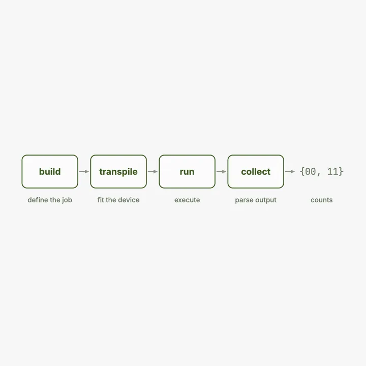
Build, transpile, run, collect. A quantum job is a pipeline, and if you ship automations you already know most of the shape.

My day job, for years, has been wiring up automations. Pipelines. Something comes in, it moves through a sequence of stages, each stage transforms it, the flaky external bits get handled, and structured output comes out the other end. I have built a lot of these, and the shape is burned into how I think.
The first time I ran a real quantum job, end to end, I had a small jolt of recognition. It is the same shape. Define the work, adapt it to the machine that will run it, execute it while handling the parts that are unreliable, collect and parse the output. That reframe did more to make the Qiskit runtime click for me than any amount of physics. So here is a quantum job as what it actually is to a builder: a pipeline.
Every pipeline has the same four stages
Strip any automation down and you find the same skeleton. You define the work, declaratively, as a description of what should happen. You adapt that description to whatever system is going to run it, because the abstract plan is never quite what the runner wants. You execute, and executing means dealing with retries, rate limits, and things that fail. And you collect the output and parse it into whatever comes next.
A quantum job has exactly these four stages, and naming them that way takes most of the mystery out. Build, transpile, run, collect. Let me walk each one in those terms.
Stage one: build is defining the job
The quantum circuit is your job definition. It is declarative, the same way a good pipeline config is declarative: you describe the operations and their order, you do not micromanage the execution. Gates in sequence, then measurement.
from qiskit import QuantumCircuit

qc = QuantumCircuit(2, 2)
qc.h(0)                  # the work, described
qc.cx(0, 1)
qc.measure([0, 1], [0, 1])
This is the entangling circuit from the entanglement post, but the point here is not what it computes, it is what it is. It is a specification. Nothing has run. You have written down the work, exactly as you would define a workflow before any of it executes. Clean separation between describing and doing, which is the first thing any pipeline gets right.
Stage two: transpile is adapting to the target
Your circuit is abstract. It uses whatever gates were convenient to think in. The machine that runs it, real or simulated, has its own fixed set of operations it can actually perform. So before it can run, the circuit has to be rewritten into the target's native operations. That is transpilation, and if you have ever had a build step that compiles or adapts your job for a specific runner, you already understand it.
from qiskit import transpile

native = transpile(qc, basis_gates=["rz", "sx", "x", "cx"], optimization_level=1)
print(sorted({instr.operation.name for instr in native.data}))   # ['cx', 'measure', 'rz', 'sx']
Run it. The Hadamard you wrote is gone, recompiled into the gates this target actually supports, and the transpiler has quietly tried to optimise the circuit while it was at it. This is exactly the compile for the target step in any deployment.
One thing to be clear about, because it matters later. That list of four gates is a target I invented for the example. A real device does not let you choose: it publishes its own native gate set, and yours may not contain a CNOT at all. Several current IBM machines implement CZ instead, so a CNOT you write gets rewritten into a CZ wrapped in single qubit rotations before it ever reaches the chip. When you compile for real hardware you hand the transpiler the backend's own target rather than a hand written list, and it uses that machine's gates, its qubit connectivity, and its error rates to decide what your circuit becomes. Same step, better informed. A local simulator and a real device get compiled differently for the same reason you build differently for staging and production.
Stage three: run through a primitive is execution
Now you execute, and modern Qiskit runs jobs through a primitive, the object from the version trap post. There are two. A Sampler when you want the measurement outcomes, the counts. An Estimator when you want a single expectation value. For a circuit with measurements and a distribution to collect, you reach for the Sampler.
The execution parameter that will feel most familiar is shots. A quantum result is a distribution, not a single value, so you run the circuit many times and tally the outcomes, and shots is how many times. It is your sample size. More shots, a cleaner estimate of the distribution, at the cost of more runtime. If you have ever tuned a batch size or a sample count against a time budget, this is the same dial.
The other familiar idea is environments. Running on a local simulator is your dev environment: fast, free, deterministic in its distribution, always available. Running on real hardware through the cloud runtime is production: there is a queue, you wait your turn, it costs real time, and the results come back noisy because a physical device is an imperfect machine. Treating the simulator as dev and the hardware as prod, and not being surprised when prod is slower and messier, is exactly the right instinct.
Stage four: collect and parse the output
The job finishes and hands back a structured result, and you parse it the way you parse any API response: reach into the known shape and pull out the field you want. For a Sampler, the counts live under the classical register you measured into.
from qiskit.primitives import StatevectorSampler

result = StatevectorSampler().run([native], shots=1024).result()
counts = result[0].data.c.get_counts()
print(counts)   # {'00': ~512, '11': ~512}
Run it. You index the result for your circuit, reach into its data, name the register, and get the counts dictionary back. This is the .c versus .meas gotcha from the version trap post, and it is the same care you take parsing any structured response: know the shape, name the field correctly, do not assume. Out comes a clean dictionary you can feed into whatever happens next.
The whole pipeline, in one piece
Put the four stages together and the job reads like any pipeline you have written.
from qiskit import QuantumCircuit, transpile
from qiskit.primitives import StatevectorSampler

# 1. build: define the work
qc = QuantumCircuit(2, 2)
qc.h(0); qc.cx(0, 1)
qc.measure([0, 1], [0, 1])

# 2. transpile: adapt to the target
native = transpile(qc, basis_gates=["rz", "sx", "x", "cx"], optimization_level=1)

# 3. run: execute through a primitive
result = StatevectorSampler().run([native], shots=1024).result()

# 4. collect: parse the structured output
print(result[0].data.c.get_counts())   # {'00': ~512, '11': ~512}
Run it. Build, transpile, run, collect. The Bell correlation comes out the end as a tidy dictionary, only 00 and 11, just as the entanglement post promised. Nothing about the flow is exotic. It is the pipeline skeleton you already know, with quantum work in the middle.
When the output is a metric, not rows
Sometimes a pipeline does not return a table of records, it returns a single aggregate, a KPI, one number that summarises the run. Quantum jobs have that mode too, and it is the second primitive. The Estimator does not give you counts, it gives you an expectation value, one number summarising a property of the state.
from qiskit.primitives import StatevectorEstimator
from qiskit.quantum_info import SparsePauliOp

bell = QuantumCircuit(2); bell.h(0); bell.cx(0, 1)
value = StatevectorEstimator().run([(bell, SparsePauliOp("ZZ"))]).result()[0].data.evs
print(float(value))   # 0.9999999999999998, which is 1 up to floating point
Run it. You get one, as close to it as floating point allows, which is the perfectly correlated answer for the Bell state: the two qubits always agree, so the ZZ correlation is maximal. That trailing rounding error is worth noticing rather than ignoring, because it is the first hint of something the algorithm posts will keep running into: expectation values arrive as floating point numbers and you compare them with a tolerance, never for exact equality. Notice also that there is no measurement on the circuit and no counts to parse, just a number out. So the rule mirrors ordinary pipelines. Want the full distribution, the rows? Sampler. Want one summary metric? Estimator. Choosing the right primitive is the same call as choosing whether your job emits records or a single computed figure, and getting it right keeps the rest of the flow clean.
Batching: many circuits, one job
Every primitive takes a list, not a single circuit, and that is not incidental. It is batching, the same instinct you use to amortise overhead anywhere: send many units of work in one job instead of paying the round trip cost over and over.
a = QuantumCircuit(1, 1); a.h(0); a.measure(0, 0)
b = QuantumCircuit(1, 1); b.x(0); b.measure(0, 0)

result = StatevectorSampler().run([a, b], shots=1000).result()
print(result[0].data.c.get_counts())   # {'0': ~500, '1': ~500}
print(result[1].data.c.get_counts())   # {'1': 1000}
Run it. Two circuits, one job, and you index the result by position to get each one's counts back, the first a fifty fifty superposition and the second a certain 1. On real hardware this matters even more than locally, because each submission waits in a queue, so bundling related circuits into one job is the difference between waiting once and waiting ten times. If you have ever batched API calls to dodge rate limits, you already have the instinct. It transfers directly.
Observability: inspect before you run
The last habit any serious pipeline has is looking before you leap. You do not fire a job blindly into production, you inspect what you are about to send, its size, its cost. A transpiled circuit tells you the same things, and you should read them before spending a slot on real hardware.
qc = QuantumCircuit(2); qc.h(0); qc.cx(0, 1); qc.measure_all()
native = transpile(qc, basis_gates=["rz", "sx", "x", "cx"], optimization_level=1)
print("depth:", native.depth(), "ops:", dict(native.count_ops()))
# depth: 5 ops: {'rz': 2, 'measure': 2, 'sx': 1, 'cx': 1, 'barrier': 1}
Run it. You see the depth, how many sequential layers the circuit is, and the operation counts. The barrier in there is not a gate, it is a marker that measure_all inserts to stop the transpiler from optimising across the measurement, and seeing things in the output that you did not write yourself is itself part of the lesson: what you built and what actually gets sent are two different objects.
On a noisy device these numbers are your cost and risk estimate: more depth means more time for the qubits to decohere, which a later post gets into, and more two qubit gates means more error, because those are the expensive, error prone ones. Reading the transpiled circuit before running it is exactly the observability step of logging a compiled job before you ship it. You find out what you actually built, and roughly what it will cost, while it is still cheap to change your mind.
Parameterised circuits: a job template with inputs
One more pattern that maps cleanly. Often you do not want a single fixed job, you want a template with a variable you fill in at run time, the same circuit run at many settings. Qiskit supports exactly this with parameters: you leave a value symbolic when you build, and bind it just before running.
import numpy as np
from qiskit.circuit import Parameter

theta = Parameter("theta")
qc = QuantumCircuit(1, 1)
qc.ry(theta, 0)          # a rotation by an angle you have not chosen yet
qc.measure(0, 0)

runs = [qc.assign_parameters({theta: 0.0}), qc.assign_parameters({theta: np.pi})]
result = StatevectorSampler().run(runs, shots=1000).result()
print(result[0].data.c.get_counts())   # theta=0  -> {'0': 1000}
print(result[1].data.c.get_counts())   # theta=pi -> {'1': 1000}
Run it. The circuit was built once with the angle left open, then bound to two values and run as one batched job, giving a certain 0 at angle zero and a certain 1 at angle pi. This is the job template with variables that every pipeline person knows: define the shape once, parameterise the part that varies, sweep the values. It is the backbone of the variational algorithms, where an optimiser tunes the parameters between runs to search for an answer, but the pattern itself is the plain one you already use whenever you run the same workflow across a range of inputs.
The instincts that transfer, and the one that does not
Most of what I know about running pipelines carried straight over. Batching: you hand the primitive a list of circuits because you can run many in one job, the same way you batch work to amortise overhead. Environments: simulator is dev, hardware is prod, and you debug on the cheap one before you spend on the slow one. Observability: you inspect the transpiled circuit before running it, the way you would log the compiled job before shipping it, so you can see what actually got sent. Unreliable dependencies: hardware noise is the flaky external service you design around, with more shots and error mitigation, the statistical corrections applied after the run, instead of naive retries.
But I want to be honest about where the analogy breaks, because oversold analogies do damage. In an ordinary pipeline you can inspect any intermediate value, log it, print it, set a breakpoint and look. You cannot do that inside a quantum circuit. Measuring an intermediate state collapses it and destroys the computation, so there is no print debugging in the middle, no peeking at the qubits mid flight. And the output is fundamentally a distribution, not a single deterministic value, so you think in shots and statistics rather than exact returns. The skeleton is the same. The thing flowing through it obeys different rules, and pretending otherwise will mislead you. Know the shape that transfers and the substance that does not.
A quick test before you move on
Close this and answer in your own words.
What are the four stages of a quantum job, and what does each one correspond to in an ordinary pipeline? If you cannot get build, transpile, run, collect and tie each to something familiar, reread the four stages.
What does the shots parameter control, and what is the everyday analogy? If sample size is not in your answer, go back to the execution stage.
Why do you hand a real backend's target to the transpiler instead of a list of gates you chose yourself? If the machine's own gates, connectivity and error rates are not in your answer, reread the transpile stage.
And where does the pipeline analogy break down? If you cannot name that you cannot inspect intermediate state and that the output is a distribution, reread the section on the instincts that transfer, because that is the part that keeps the analogy from misleading you.
Where I am learning it
Free, and this is the part where my existing world and the new one overlap most, so it went quickly. The Qiskit documentation on primitives and on the runtime is the current, versioned source for how jobs actually run, and unlike a lot of older material it is built around exactly this build, transpile, run shape. The local primitives, the ones in the examples here, run on your own machine for free, which makes them the perfect dev environment to practise the whole flow in before you ever touch a real device or its queue. As always, I learned it by running it, because a pipeline I have only read about is not one I trust until I have watched my own output come out the end of it. Every output comment in this post is what my machine actually printed, floating point noise included, apart from the ones marked with a tilde, which are typical values because sampling varies from run to run.
The runtime stopped being foreign
The cloud runtime, the primitives, the transpilation step, all of it looked like a new and intimidating system when I started, a pile of quantum specific machinery I would have to learn from scratch. It is a pipeline. Define the work, adapt it to the target, execute it while handling the unreliable parts, collect and parse the output. I have built that shape a hundred times in a completely different domain, and the shape did not change just because the work in the middle turned quantum.
That is the quiet advantage of coming to this as a builder. The physics is genuinely new and you have to earn it. But a surprising amount of the surrounding engineering is not new at all, it just wears unfamiliar names. Recognising the pipeline under the runtime is worth more than it sounds, because it means your instincts are more transferable than the vocabulary lets on. Mine were. Yours probably are too.