Deutsch Jozsa: the hello world of quantum advantage
Constant or balanced in a single evaluation. The first algorithm where quantum genuinely beats classical, built from scratch.

This is the first algorithm where a quantum computer genuinely beats a classical one, and it is simple enough to build by hand in a few lines. The problem it solves is a toy, completely useless in practice, and I will be honest about that. But the toy is doing something real, and watching it work is the first time the abstract promise of quantum advantage turns into a concrete thing you can run. It is the hello world of the whole field.
The problem
You are handed a function. It takes a bit string and returns a single bit, 0 or 1. You cannot look inside it, you can only feed it inputs and see outputs. And you are given a promise: the function is one of exactly two kinds. Either it is constant, meaning it returns the same value for every possible input, all zeros or all ones. Or it is balanced, meaning it returns 0 for exactly half of the inputs and 1 for the other half. Your job is to find out which kind it is. Constant or balanced. That is the whole question.
What it costs classically
Think about how you would do this with an ordinary computer. You feed in one input and look at the output. Say you get 0. Does that tell you anything? Almost nothing. The function could be constant, always returning 0, or it could be balanced and you happened to hit one of its 0 inputs. You try another input. Still 0. Still ambiguous, it could be a constant 0 or a balanced function whose 0 half you keep landing in.
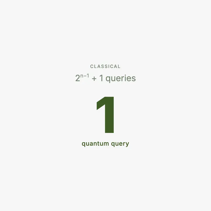
To be certain, you have to keep going until you either see a 1, which instantly proves it is not constant 0, or until you have checked just over half the inputs all returning the same value, at which point it cannot be balanced and must be constant. For an n bit input there are 2 to the n possible inputs, and in the worst case you need to check half of the 2 to the n inputs, plus one, to be sure. For a 20 bit function that is over half a million queries, just to answer one yes or no question. Classically, you cannot do better in the worst case, because a balanced function can disguise itself as constant for exactly half its inputs.
It is worth seeing exactly why that half plus one is the magic number. Suppose you have checked half of all the inputs and every one returned 0. You still cannot conclude constant, because a balanced function is allowed to return 0 on exactly half its inputs, and you might have hit precisely that half. Only when you check one more, the half plus one input, and it too returns 0, can you be sure, because a balanced function could not have given 0 to more than half. So the worst case is genuinely half the inputs plus one, and an adversary choosing the function could always force you to that worst case. There is no cleverness that escapes it classically, because each query reveals the value at one input and nothing about the others, and you simply need enough values to rule out the disguise.
What it costs on a quantum computer
One query. Always. No matter how many input bits. You evaluate the function a single time, in superposition, and the answer falls out. That is the separation: over half a million classical queries collapse to one quantum query. For this contrived problem, the gap between classical and quantum is as stark as it ever gets.
Building it
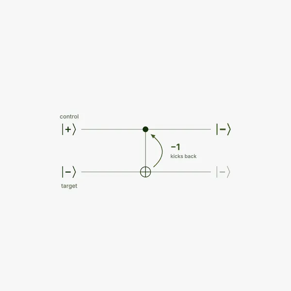
The circuit is short and it is pure phase kickback from the last post. You take some input qubits and one ancilla qubit. You put the ancilla into the |−⟩ eigenstate, you put the inputs into a superposition of all possible inputs with Hadamards, you apply the oracle once, you apply Hadamards to the inputs again, and you measure the inputs. Here is the whole thing for a three bit input.
from qiskit import QuantumCircuit
from qiskit.primitives import StatevectorSampler

def deutsch_jozsa(oracle, n=3):
    qc = QuantumCircuit(n + 1, n)
    qc.x(n); qc.h(n)               # ancilla -> |->
    for q in range(n):
        qc.h(q)                    # inputs -> superposition of everything
    oracle(qc, n)                  # query the function, once
    for q in range(n):
        qc.h(q)                    # interfere
    qc.measure(range(n), range(n))
    return qc

# a constant function: f(x) = 0 for all x, so the oracle does nothing
constant = deutsch_jozsa(lambda qc, n: None)

# a balanced function: CNOT each input into the ancilla
def balanced_oracle(qc, n):
    for q in range(n):
        qc.cx(q, n)
balanced = deutsch_jozsa(balanced_oracle)

sampler = StatevectorSampler()
print("constant ->", sampler.run([constant], shots=1000).result()[0].data.c.get_counts())
print("balanced ->", sampler.run([balanced], shots=1000).result()[0].data.c.get_counts())
Run it. The constant function returns all zeros, 000, every single time. The balanced function returns something that is not all zeros, here 111 every time, always the same string because this particular balanced oracle, a CNOT from every input, is the parity function, and the closing Hadamards land all of its weight on one outcome. And there is your answer, read off in one query: measure all zeros and the function is constant, measure anything else and it is balanced. One query each, and the two cases are perfectly distinguishable. The decision rule is that simple. All zeros means constant. Anything else means balanced.
The original, on a single bit
It helps to shrink the problem to its smallest form, which is also the historical original, the version Deutsch published before Deutsch and Jozsa generalised it. One input bit. A function from one bit to one bit. There are exactly four such functions, and they split neatly into the two camps. Two are constant: the one that always returns 0, and the one that always returns 1. Two are balanced: the one that returns its input unchanged, and the one that returns the opposite of its input. Constant or balanced, two of each, and the question is which camp your mystery function is in.
def deutsch1(oracle):
    qc = QuantumCircuit(2, 1)
    qc.x(1); qc.h(1)        # ancilla -> |->
    qc.h(0)                 # the one input qubit -> superposition
    oracle(qc)
    qc.h(0)
    qc.measure(0, 0)
    return qc

const_0  = deutsch1(lambda qc: None)         # f(x) = 0
const_1  = deutsch1(lambda qc: qc.x(1))      # f(x) = 1
balanced = deutsch1(lambda qc: qc.cx(0, 1))  # f(x) = x

for name, qc in [("constant 0", const_0), ("constant 1", const_1), ("balanced", balanced)]:
    counts = sampler.run([qc], shots=500).result()[0].data.c.get_counts()
    print(f"{name:12} -> {counts}")
Run it. Both constant functions, the always 0 and the always 1, measure 0. The balanced function measures 1, and so would the other balanced one, since flipping the output only adds a global phase. So on a single bit the rule is even starker: measure 0, the function is constant, measure 1, it is balanced, and one query settles it. Classically, on one bit, you would need two queries to be sure, since a single query never rules out the other camp. Quantum needs one. The separation is small here, two versus one, but it is the seed of the dramatic gap that opens up as the input grows, and it is the cleanest case to trace by hand.
Why it works
The mechanism is the two beat rhythm from the kickback post, and it is worth walking because it is the same rhythm every later algorithm uses. The opening Hadamards put the input register into an equal superposition of every possible input at once, so the single oracle call effectively sees all inputs simultaneously. The ancilla sits in |−⟩, so the oracle does not write f's values into an output, it kicks them back as phases onto the input superposition. After the oracle, the function's entire behaviour is encoded in the pattern of phases across the inputs, invisible to a measurement but fully present.
Then the closing Hadamards interfere those phases, and this is where the magic resolves into mechanics. If the function is constant, every input got the same phase, so the phases are all aligned, and when you interfere aligned phases they reinforce back into the all zeros state with certainty. If the function is balanced, the phases form a pattern that is, in a precise sense, the opposite of aligned, and interference sends the result anywhere except all zeros. So the final measurement is really asking one question of the phases: did they all agree? Constant functions make them agree and you read 000. Balanced functions make them disagree and you read something else. The algorithm detects a global property of the entire function, its constant ness or balanced ness, in a single query, by stamping f into phases and letting interference judge whether they line up.
It is worth grounding alignment and opposition with the smallest multi bit case, two input bits. There are four inputs, 00, 01, 10, 11. A constant function gives them all the same value, so kickback stamps them all with the same phase, four phases pointing the same way. When the Hadamards interfere four aligned phases, they add up constructively on the all zeros outcome and cancel everywhere else, so you measure 00 with certainty. A balanced function gives 0 to two of the inputs and 1 to the other two, so kickback stamps two of them with one phase and two with the opposite phase. Now the phases are split half and half, and when interference combines a perfectly balanced split like that, the all zeros outcome cancels to nothing while weight piles up elsewhere, so you are guaranteed to measure something other than 00. That is the precise meaning of aligned versus opposed: constant means every phase agrees and they reinforce into all zeros, balanced means the phases cancel out the all zeros outcome exactly. The single measurement is reading the result of that interference, which is reading a global fact about all four function values at once.
The honest caveat
I promised honesty, so here it is plainly. This problem is useless. Nobody, anywhere, needs to know whether a mystery function is constant or balanced under a promise that it is exactly one of those two. It is a contrived setup, built specifically to have a clean quantum win, exactly the kind of contrived advantage the NISQ post warned you to be sceptical of. Deutsch and Jozsa did not give us a tool. They gave us a proof of principle, the first clean demonstration that a quantum computer can, on some problem, do dramatically less work than any classical one.
One more piece of honesty, the same one the first badge post insisted on: the exponential gap holds against exact classical algorithms only. Allow the classical machine to be randomised and to accept a small chance of being wrong, and it solves the same problem in a handful of queries.
That proof of principle matters, because the mechanism is not contrived even though the problem is. Superposition to see all inputs at once, phase kickback to write the function's answer into phase, interference to extract a global property in one shot, that machinery is exactly what the genuinely interesting algorithms use too. The problem is a toy. The engine is the real thing. Learning it here, where everything is small and you can run it and read every line, is how you come to understand the engine before meeting it inside something harder.
It is also worth knowing the historical weight of this little algorithm, because it earned its place. When Deutsch and Jozsa published it, it was the first clean proof that a quantum computer could provably outperform a classical one on a well defined task, with certainty rather than just on average. That was not obvious beforehand, and it mattered enormously as a proof of concept that the whole field could be built on. It directly inspired the algorithms that came after, Bernstein and Vazirani next, and then the genuinely powerful ones, each one borrowing and extending the superposition, kickback, interference pattern that this toy demonstrated first. So when you run it, you are running the algorithm that convinced people quantum advantage was real at all. The problem it solves is useless, and it changed the trajectory of the field anyway, precisely because it showed the mechanism could work. That is a strange and instructive combination, and a reminder that a result can be practically worthless and historically pivotal at the same time.
A quick test before you move on
Close this and answer in your own words.
What are the two kinds the mystery function might be, and what is the decision rule from the measurement? If you cannot say constant or balanced, and all zeros means constant, reread the problem and the build sections.
Why does a constant function interfere back to all zeros while a balanced one does not? If aligned phases reinforce, opposed phases scatter is not roughly your answer, revisit the why it works section.
And why is this algorithm a proof of principle rather than a useful tool? If you cannot explain that the problem is contrived but the mechanism is real, reread the honest caveat, because holding both at once is the whole point.
Where I am learning it
Free. Deutsch and Jozsa is in essentially every quantum algorithms course and in the IBM Quantum learning materials, and it is the right first algorithm because it is small enough to hold entirely in your head. The thing that taught me most was swapping in different oracles, a constant one, a few different balanced ones, and confirming each time that constant gives all zeros and balanced never does. As always, the algorithm did not feel real until I ran it myself and watched one query decide a question that would cost a classical computer a fortune.
The first taste
Deutsch and Jozsa is a toy, and I would rather say that plainly than dress it up. But it is the first place the promise of quantum computing stops being a slogan and becomes something you can build and run in ten lines, where one query does what classical computing needs half a million to do. The win is real even if the problem is not.
And the move it teaches is the move. Put everything in superposition, use phase kickback to write the answer into phase, interfere to read out a global property in a single shot. Every algorithm worth knowing is a richer version of exactly this. You have now run the simplest one end to end, which means the harder ones are not a different language. They are this, with more to say.