Three quantum ways to diagonalise a giant matrix
A surprising number of hard problems are one eigenvalue problem on a matrix too big to build. Variational, Krylov, sample based, compared.

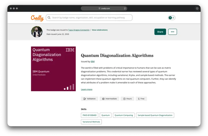
A surprising number of the hard problems people actually want a quantum computer for are the same problem underneath. Find the lowest eigenvalue of a very large matrix. The energy of a molecule in its ground state, the behaviour of a new material, certain optimisation problems, all of them reduce to one task: build a large Hermitian matrix, one equal to its own conjugate transpose, called a Hamiltonian, then find its smallest eigenvalue and the vector that produces it. The badge behind this post, IBM's Quantum Diagonalization Algorithms, is about the quantum algorithms built for exactly that, and there are three families worth telling apart.
One problem wearing many costumes
The matrix in question is a Hamiltonian, the object that encodes a system's energy. Its eigenvalues are the allowed energies, and the smallest one is the ground state energy, the lowest the system can sit at. For chemistry that ground state energy is the prize, because it decides how molecules bond and react. The whole game, across chemistry and materials and more, is reading one number off a matrix: the bottom eigenvalue. Diagonalising a matrix means finding its eigenvalues, and for small matrices that is a solved, boring problem. The trouble is the size.
Why you cannot just diagonalise it
The matrix for n qubits is 2ⁿ by 2ⁿ. That exponential is what makes this hard. For 10 qubits the matrix is 1024 by 1024, which a laptop diagonalises instantly. For 50 qubits it is over a quadrillion by a quadrillion, and there is not enough memory on Earth to even write it down, let alone diagonalise it. Classical exact diagonalisation, the function I am about to use on a toy, simply stops being possible somewhere around twenty qubits. Everything in this badge is a strategy for getting the bottom eigenvalue of a matrix you can never hold in memory.
The honest small example
To make the rest concrete I need a matrix small enough to diagonalise the old fashioned way, so I have an answer key to check the clever methods against. Here is a real one, two qubits, a pair of coupled spins.
import numpy as np

X = np.array([[0, 1], [1, 0]], dtype=complex)
Y = np.array([[0, -1j], [1j, 0]], dtype=complex)
Z = np.array([[1, 0], [0, -1]], dtype=complex)

H = np.kron(X, X) + np.kron(Y, Y) + np.kron(Z, Z)   # 4x4 Hamiltonian
evals = np.linalg.eigh(H)[0]
print(np.round(evals, 3))      # [-3.  1.  1.  1.]
Run it. The eigenvalues are -3, 1, 1, 1, so the ground state energy is -3. That is the number every method below is trying to recover without the luxury of building H and calling eigh on it. And there is a detail I did not expect the first time I saw it. The ground state, the vector with energy -3, is the singlet, (|01⟩ - |10⟩)/√2, which is an entangled state. The lowest energy configuration of two coupled spins is not either spin pointing in some definite direction. It is the two of them entangled. Entanglement, which had only come up in passing so far, turns out to be where the energy is minimised, which is a quiet and satisfying link between two things I had learned as if they were separate.
Variational: guess, measure, adjust
The first family is the variational one, and it rests on a single guarantee from physics: the average energy of any state you can prepare is never lower than the true ground energy. So you build a circuit with adjustable knobs, a parameterised state |ψ(θ)⟩, measure its average energy, and let a classical optimiser turn the knobs to push that number down. The lowest you can drive it is your estimate of the ground energy. Here is that loop against the toy Hamiltonian, the same H written as a sum of Pauli terms, the X, Y and Z matrices from the first block, with a small two qubit circuit and an ordinary optimiser, run on a simulator.
import numpy as np
from qiskit.circuit import QuantumCircuit, Parameter
from qiskit.quantum_info import SparsePauliOp, Statevector
from scipy.optimize import minimize

H = SparsePauliOp(["XX", "YY", "ZZ"], coeffs=[1, 1, 1])   # XX + YY + ZZ

a, b, c, d = (Parameter(p) for p in "abcd")
ansatz = QuantumCircuit(2)                 # the adjustable knobs
ansatz.ry(a, 0); ansatz.ry(b, 1)
ansatz.cx(0, 1)
ansatz.ry(c, 0); ansatz.ry(d, 1)

def energy(x):                             # average energy of the prepared state
    state = Statevector(ansatz.assign_parameters(dict(zip([a, b, c, d], x))))
    return float(np.real(state.expectation_value(H)))

rng = np.random.default_rng(0)
best = min((minimize(energy, rng.uniform(0, 2 * np.pi, 4), method="COBYLA")
            for _ in range(20)), key=lambda r: r.fun)
print("VQE ground energy:", round(best.fun, 3))   # -3.0
Run it. The optimiser drove the energy down to -3.0, landing on the exact ground value. This is VQE, the variational quantum eigensolver, and its shape is a parameterised pipeline: define the circuit once, leave the angles open, sweep them. The difference from a plain sweep is that here an optimiser chooses the next angles based on the last measured energy. The quantum computer prepares states and reports their energy. The classical computer decides where to look next. The work is split between the two, and that division is the whole character of this style of algorithm.
Krylov: build a tiny good subspace
The second family is quieter and, to me, more elegant. The full space is impossibly large, but the ground state usually lives in a tiny, well chosen corner of it. Krylov methods build that corner on purpose. Starting from some state |ψ⟩, you generate a small handful of related states by applying the Hamiltonian again and again, |ψ⟩, then H|ψ⟩, then H²|ψ⟩, and so on, which tends to pull the set toward the extreme ends of the spectrum, the lowest energies and the highest ones alike. Then you diagonalise the Hamiltonian only inside that small subspace, a tiny matrix you can handle, and its lowest eigenvalue approximates the true one. On a quantum computer the subspace is built from states evolved under the Hamiltonian for a few short times rather than from powers of H, and the small matrix is filled in by measuring overlaps between them, which is the step a classical machine cannot afford at scale. Here it is on the toy, with a two dimensional subspace built from a start vector and one application of H.
import numpy as np
from qiskit.quantum_info import SparsePauliOp

H = SparsePauliOp(["XX", "YY", "ZZ"], coeffs=[1, 1, 1]).to_matrix()

rng = np.random.default_rng(1)
v = rng.normal(size=4); v = v / np.linalg.norm(v)              # needs nonzero ground state overlap
w = H @ v; w = w - np.vdot(v, w) * v; w = w / np.linalg.norm(w)  # one step, orthogonalised
K = np.column_stack([v, w])                                    # the 2 dim subspace

H_small = K.conj().T @ H @ K                                   # H restricted to it
print("Krylov ground energy:", round(float(np.linalg.eigvalsh(H_small)[0]), 3))  # -3.0
Run it. That two by two problem returns -3.0 exactly, the same answer the full matrix gave. Do not read too much into the word exactly, because this toy is easier than it looks. My Hamiltonian has only two distinct eigenvalues, -3 and 1, so a two dimensional Krylov space is already guaranteed to hold the ground state component in full. On a real Hamiltonian with a dense spectrum you get an approximation that tightens as the subspace grows, and that is the honest version of the trade. The trade is the heart of it. You replace one impossible diagonalisation with one easy diagonalisation, on a subspace small enough to be classical, and you accept an approximation that improves as the subspace grows. There is no optimiser searching here. You are constructing a good basis and then solving exactly inside it.
The start vector is not free either. Krylov can only reach what the first vector already touches, so a start state with no overlap at all on the ground state leaves the method stuck forever. On this Hamiltonian |00⟩ is exactly that trap: it is a triplet state, one of the three states with energy 1, orthogonal to the singlet, so the subspace collapses to a single vector and the method reports 1 instead of -3. A random start avoids that with probability one, which is why the code uses one.
Sample based diagonalisation: let the hardware choose the basis
The third family is the newest, and it is the one that fits my own instincts best, because it is a clean division of labour between a quantum machine and a classical one. The idea, called sample based quantum diagonalisation, goes like this. Run a quantum circuit and measure it many times. The bitstrings that come back most often point to the configurations that matter most for the ground state. Collect those few important configurations, build the Hamiltonian restricted to just that small set, and diagonalise that small matrix on a classical computer. Then feed what you learned back in and repeat.
The quantum computer is doing the one thing it is good at, exploring an enormous space and reporting which corners are worth looking at. The classical computer is doing the one thing it is good at, exactly diagonalising a small, well chosen matrix. Neither could do the job alone at scale, and the method is built around handing each part to the machine suited for it. As someone whose day work is wiring systems together so each piece does what it does best, this is the algorithm in the badge that felt the most like home.
What this badge says, and what it does not
The badge, Quantum Diagonalization Algorithms, is an intermediate one, and the honest reading of it is this. It certifies that I worked through IBM's coursework on quantum diagonalisation, that I understand the variational, Krylov, and sample based families, and that I can reason about which kind of problem suits which approach. The toy calculations above are mine, run on my own machine, and they are reproducible.
The official badge description also says the earner can implement these algorithms on real quantum computers. I want to be careful and exact about that line. The course does cover implementation on real backends, and the small versions above I have run in simulation. My own first run on a real quantum processor is a separate milestone, and it is one I have not published yet. I am not going to let a badge's wording quietly promote a simulator result into a hardware result. The understanding is real and earned. The hardware run is still ahead of me, and when I do it, it gets its own honest post.
Where I am learning it
Free, through IBM Quantum Learning on the open plan, IBM's free tier, with the interactive labs and the verifiable badge at the end. The diagonalisation course is the source for the three families above. As in the earlier posts where I built things, the part that actually taught me was building the toy myself, computing the answer key with plain linear algebra, and then watching each method recover that same number a different way. Three roads to one eigenvalue is a far clearer lesson when you have walked two of them in code on a problem small enough to check by hand.
Three roads, one number
The thing I am taking from this badge is not three algorithms as separate recipes. It is one problem, find the bottom of a matrix too big to build, approached three ways that differ only in how they beat the size. Variational searches with an optimiser. Krylov constructs a small honest subspace. Sample based lets the hardware vote on which corners matter and hands the rest to a classical solver. Different instincts, same target, and knowing which instinct fits a given problem is most of the skill.
The matrix was too big to ever write down. The answer was a single number at the bottom of it. Most of quantum computing, it turns out, is clever ways of reaching that number without ever holding the matrix.