I ran a Bell state on real IBM quantum hardware

Most of the code in this series so far ran on a simulator. A perfect, noiseless, mathematical model of a quantum computer, living on my own machine, where the answer comes out exactly as the math says it should. That was the right place to learn. It is not where quantum computers actually are.

This time I did something different. I took the simplest entangled circuit, the Bell state from a few posts back, and I ran it on a real quantum computer. An actual chip, cooled to near absolute zero, sitting in an IBM lab, reached over the internet. The result was not perfect. Then I did the part that most first hardware posts skip: I opened the machine's own calibration data and worked out where every wrong answer came from.

The circuit, and the perfect answer

Here is the circuit. It is the same two gates as the entanglement post: a Hadamard, then a CNOT, then measure both qubits.

from qiskit import QuantumCircuit
from qiskit.primitives import StatevectorSampler

qc = QuantumCircuit(2, 2)
qc.h(0); qc.cx(0, 1)
qc.measure([0, 1], [0, 1])

ideal = StatevectorSampler().run([qc], shots=4096).result()[0].data.c.get_counts()
print(ideal)   # only '00' and '11', about 2048 each

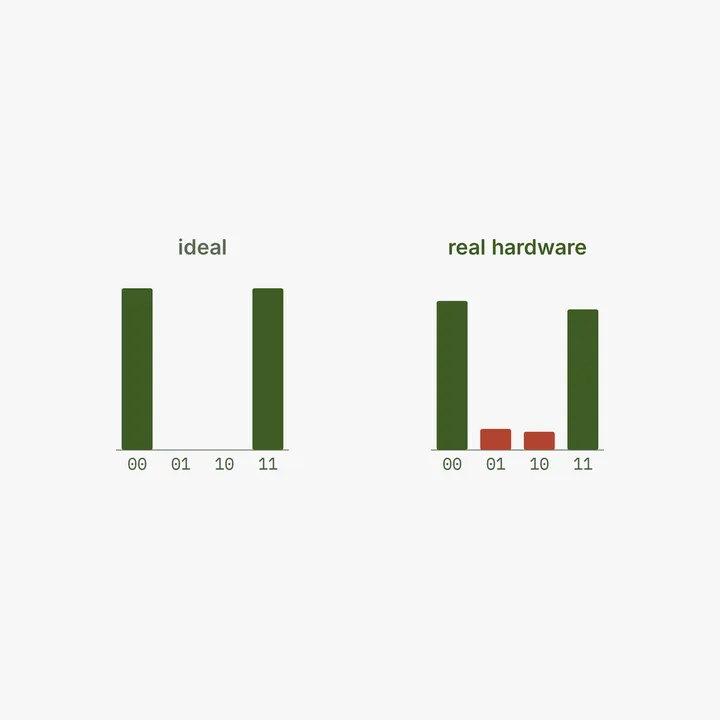
Run it. On the simulator you get only 00 and 11, split roughly evenly, and nothing else. The two qubits always agree, exactly as the Bell state promises. Zero counts on 01 and 10, the outcomes where the qubits disagree, because in the ideal state those outcomes have zero amplitude. Hold this clean result in mind. It is the reference the real machine is about to be measured against.

Getting onto a real machine

IBM gives free access to real quantum hardware over the cloud, through the Qiskit Runtime. The flow is the pipeline from the earlier post, with the target swapped from simulator to a physical device. You connect to the service, pick a backend, transpile your circuit for that specific machine's native gates and layout, submit the job, and wait in a queue behind everyone else on Earth doing the same thing. Then the results come back.

I will not paste my credentials and connection boilerplate here, because that part is just setup and the IBM docs cover it better than I could. The conceptual shift is the only thing that matters: this is the pipeline going to production. The simulator was your dev environment, free and instant and perfect. The real device is prod, with a queue, a cost in wait time, and output that reflects the messy physics of an actual machine. The code shape barely changes. What changes is that the universe is now doing the computing, and the universe is noisy.

The connection, in shape

Even though I will skip my account specifics, the shape of the code is worth seeing once, because it is almost identical to the local pipeline. You connect to the runtime service, ask it for a real backend, compile your circuit specifically for that machine, and run it through a Sampler, exactly the same primitive as before, just pointed at hardware instead of a simulator.

# requires the qiskit-ibm-runtime package and your own IBM Quantum account
from qiskit_ibm_runtime import QiskitRuntimeService, SamplerV2
from qiskit.transpiler.preset_passmanagers import generate_preset_pass_manager

service = QiskitRuntimeService()                              # saved credentials
backend = service.least_busy(operational=True, simulator=False)

pm = generate_preset_pass_manager(target=backend.target, optimization_level=1)
isa = pm.run(qc)                                              # compile for THIS machine

sampler = SamplerV2(mode=backend)
job = sampler.run([isa], shots=4096)
counts = job.result()[0].data.c.get_counts()                  # after the queue, real data

That is the whole structure, and notice how little is new. The service and backend lines are the only genuinely hardware specific part, and they are just "log in and pick a machine." The compilation step is the transpile step from the pipeline post, except now it targets a real device's gate set and qubit layout rather than an abstract one, which is why it goes through the backend's own target rather than a hand written gate list. And the Sampler is the same primitive concept, run a list of circuits, get structured results back, just running in the cloud on a physical chip with a queue in front of it. The pipeline shape held. Only the target moved from your laptop to a refrigerator in a lab.

The real answer, on ibm_fez on 30 August 2026

The machine I got was ibm_fez, a 156 qubit Heron r2 processor, last calibrated fifty two minutes before my job ran. The compiler placed my two logical qubits onto physical qubits 23 and 22, and the finished circuit was seven layers deep: five rz rotations, three sx gates, each half of an X gate, two measurements, and exactly one two qubit gate. Here is what came back, out of 4096 shots:

00:  2078   (50.73%)
11:  1968   (48.05%)
01:    26   (0.63%)
10:    24   (0.59%)

Look at what happened. The two outcomes that are supposed to dominate still dominate, so the correlation the circuit predicts survived the trip. 00 came back somewhat more often than 11, but before reading anything into that, check it against ordinary sampling noise: the gap is under two standard deviations of what you expect when you flip a fair coin four thousand times. A small part of it is real, for a reason I get to below, but most of it is statistics, and mistaking one for the other is the easiest way to fool yourself on a first hardware run.

The number that matters is the other one. Fifty shots came back as 01 or 10. According to the ideal Bell state those outcomes have zero amplitude and cannot happen, ever, not rarely but never. The qubits disagreed, in a state where they are physically not supposed to be able to disagree. Those fifty counts did not come from the math. They came from the hardware. That little pile in the wrong bins is noise, made visible, and the rest of this post is about reading it rather than shrugging at it.

Where the wrong answers come from

Three physical imperfections produce those stray counts, and it is worth naming them because they are the whole story of why today's hardware is hard.

Gate errors. The CNOT on a real device is not the perfect matrix from the gates post. In fact my CNOT never reached the chip as a CNOT at all: the compiler rewrote it into a CZ plus single qubit rotations, because CZ is the two qubit operation this processor physically implements. Whatever it is called, it is a physical operation driven by microwave pulses, and it is slightly off every time. On my run the published error was 0.18 percent for that CZ and 0.02 percent for a single qubit sx, which is the usual ordering: the entangling gate is the expensive one, an order of magnitude worse than its single qubit neighbours.

Readout errors. When the machine measures a qubit, it sometimes misreads it, purely because reading a quantum state off real hardware is an imperfect physical measurement. My two qubits had published readout errors of 0.56 and 0.42 percent. And this error is not symmetric, which is worth pausing on. From the device's published readout figures you can build a full assignment matrix, the probability of measuring each outcome given each true state, and mine says a true 00 is misread 0.64 percent of the time while a true 11 is misread 1.42 percent of the time. More than twice as bad. The reason is physical: measurement takes time, and during that time a qubit sitting in the excited state can relax down to the ground state, whereas a qubit already in the ground state has nowhere to fall. Reading a 1 is harder than reading a 0.

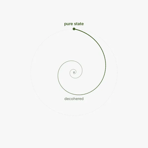
Decoherence. The qubits do not hold their state perfectly while the circuit runs. They drift, they leak, they forget. My worse qubit had a phase coherence time of 64 microseconds, and the whole circuit took 1.8 microseconds, so it spent under three percent of its coherence window alive. That is why decoherence barely registers here. It is the dominant enemy as circuits grow, and it gets its own post next, because it is the deepest reason depth is dangerous.

Every count in the wrong bin is one of these three, in physical form. The noise is not random malice. It is gate imperfection, plus readout imperfection, plus the qubits quietly decaying, all of it leaking a small fraction of your shots into outcomes the ideal math forbids.

The single qubit runs show the readout asymmetry on their own

I had spare shots in the same batch, so I ran three trivial single qubit circuits on qubit 110 as controls, and one pair of them makes the readout asymmetry visible without touching a matrix at all.

Prepare the qubit in |0⟩ and measure it 2048 times: 10 shots came back as 1, an error of 0.49 percent. Prepare the same qubit in |1⟩ on the same machine in the same batch and measure it 2048 times: 21 shots came back as 0, an error of 1.03 percent. Same qubit, same measurement, twice the error rate for the excited state, the same asymmetry the assignment matrix predicts, and for exactly the reason above.

This is the cheapest experiment in the post and one of the most useful. Two circuits with no gates worth speaking of, and they characterise the measurement itself, separately from anything your algorithm does. When a result looks wrong, knowing your readout's own error rate, per state, tells you how much of the wrongness you should have expected before you start blaming your circuit.

What this histogram does not prove

One honest caveat, because it is the thing I would have got wrong a few months ago. A histogram taken in a single measurement basis does not demonstrate entanglement. It demonstrates correlation. If someone had quietly replaced my quantum computer with a coin flip, preparing 00 half the time and 11 the other half, decided classically before anything was measured, the counts would look exactly the same as mine. Nothing in those four numbers separates a genuinely entangled state from a boring classical mixture.

What separates them is phase, and phase is invisible in this basis. The Bell state holds a definite phase relationship between its two branches that a classical mixture does not, and it shows up the moment you rotate the measurement before reading, or run a Bell inequality test, or reconstruct the state properly with tomography. That is a second experiment, and a post of its own.

So the honest reading of my run is this. I built a circuit that should produce entanglement, ran it on real hardware, and confirmed that the correlation it predicts is present, with a noise floor I can account for down to five shots. Confirming the entanglement itself needs more than one basis. Claiming it from counts like these is an easy mistake to make and a very common one to read.

You can account for most of the noise before you guess

The temptation, looking at fifty stray counts, is to shrug and say "hardware is noisy." You can do better than that, with arithmetic, and the machine hands you every input you need.

Start with readout. Both correct Bell outcomes have the two qubits agreeing, so if exactly one of them is misread, they no longer agree and the shot lands in 01 or 10. With published readout errors of 0.56 and 0.42 percent, the chance that at least one of the two is misread on a given shot is 0.97 percent, which over 4096 shots predicts about forty shots in the wrong bins.

Then the gate. This one needs a caveat, because the published CZ error is an average infidelity from benchmarking, not a probability of flipping a bit. Turning 0.18 percent of infidelity into an expected number of disagreements assumes a noise model, and the simple depolarising assumption puts the contribution on the order of 0.12 percent, roughly five shots. Treat that as an estimate with a model behind it, not a measured quantity.

Add them: about 1.09 percent predicted, and I measured 1.22 percent. The gap between the model and the measurement is 0.13 percent, five shots out of 4096. A two term back of the envelope, built entirely from numbers the machine published about itself, lands within five counts of what came back.

There is a plausible home for those last five shots, and it is worth stating as a hypothesis rather than a result. Almost all of the circuit's 1.8 microseconds is the measurement itself, and relaxation during measurement is already baked into the published readout error, which is precisely why a true 11 is misread more often than a true 00. Adding a separate decoherence term for that stretch would count the same physics twice. But the gates before the measurement take their own hundred or two hundred nanoseconds, and relaxation across that window, on qubits with these coherence times, works out to roughly a tenth of a percent. That is the order of the residual. I have not proved it is the residual, and one run cannot.

One more thing falls out of the assignment matrix. The probability of both qubits being misread on a single shot is about one in ten thousand, which over 4096 shots is a fraction of a single count, so essentially none of my noise is hiding inside 00 and 11 disguised as a correct answer. And the asymmetry from earlier shows up here too: because a true 11 is misread more often than a true 00, and because a misread 11 very occasionally lands on 00 while a misread 00 essentially never lands on 11, the measured 00 bar should sit slightly above the measured 11 bar. It does. That accounts for perhaps fifteen of the hundred and ten count gap between them. The rest really is just sampling noise.

That is the difference between watching noise and reading it. Not a clean decomposition, one run cannot prove attribution, and the model is deliberately crude. But going from "there is some noise" to "four fifths of this is the final measurement being misread, on a device whose published rates predict it to within five counts" is a diagnosis rather than a shrug.

One caveat, and it is not a small one. Those error rates are the numbers the machine published fifty two minutes before I ran. Calibration drifts. The same qubits next week are not the same qubits numerically, which means the arithmetic above has a shelf life and has to be redone against fresh device properties every time. A number you measured once and wrote down is not a number you still know.

Correcting for the readout removes most of the error

Arithmetic that predicts something should be tested by fixing that something. If four fifths of my wrong answers are the measurement being misread, then undoing the measurement error should remove four fifths of them.

The assignment matrix makes this concrete. It tells you the probability of measuring each outcome given each true state, so inverting it takes your observed counts back towards what the device most likely actually prepared. I ran a second baseline, which came back with 1.42 percent of its shots in the wrong bins, and applied the correction. The error dropped to 0.42 percent. About seventy percent of it gone, by post processing alone, no change to the circuit and no extra shots.

Two honest notes on that. First, the leftover is still around seventeen shots, roughly three times what the published CZ error on its own predicts, which is the sign that a two term budget is a simplification rather than a complete physical model. Second, this correction is a statistical estimate, not a repair. Nothing on the chip got better. I made a more informed guess about what the chip was trying to tell me, using the chip's own characterisation of how it mishears itself, and that guess can be wrong in ways the raw counts cannot.

Twirling and dynamical decoupling did nothing here

I then ran the same circuit with two techniques switched on, twirling and dynamical decoupling, half expecting an improvement to report. The wrong bins came to 1.51 percent, against 1.22 and 1.42 percent for the two baselines. It got numerically worse.

Before concluding anything from that, look at what the baselines are doing. Two identical runs, nine minutes apart, on the same machine and the same qubits, gave fifty and fifty eight wrong shots. Eight counts apart, with nothing changed between them. That spread is my measurement resolution, and the mitigated run sits four counts outside it. The correct statement is not that mitigation made things worse. It is that on this circuit, the effect of these techniques is smaller than my ability to measure it.

Which is what you should expect once you think about what each one is actually for. Dynamical decoupling protects qubits that are sitting idle while other parts of a circuit do work. My circuit is seven layers deep with one entangling gate and no idle stretches worth protecting, so there was nothing there for it to fix. Twirling is not even aimed at lowering the error rate in the first place: it converts coherent, structured errors into a well behaved random channel, which is what makes the mitigation layered on top of it statistically valid. Judging it by whether the raw count of wrong shots went down is judging it by the wrong metric entirely.

That is the real lesson, and it is why I am writing up a result that improved nothing. Error suppression is not a switch that makes results better. It is a set of tools aimed at specific failure modes, each with its own success criterion, and if your circuit does not exhibit the failure a tool targets, turning it on buys you nothing and costs you overhead. Knowing which tool addresses which failure is the actual skill. The alternative was to run it, see no improvement, quietly leave it out, and write a post implying that switching on mitigation is straightforwardly good. It is not.

The whole investigation, three jobs, cost fifteen seconds of QPU time out of the free plan's six hundred seconds per twenty eight day window. The job IDs are daa5tg1qtnsc73d298tg, daa6236rbfbs73cibee0 and daa63eerbfbs73cibfq0, in case anyone wants to check my arithmetic against the record.

What the error rate is telling you

Add up the wrong outcomes. In my first run, 01 and 10 together were 1.22 percent of all shots. That number is a rough health reading on the device and the circuit together: the fraction of results that landed where they physically should not have. For a two gate Bell state on a current Heron processor, on a good day, that is about what you should expect, and it varies with the machine, the qubits you happen to be given, and the hour.

It is a number worth computing every time you run, because it calibrates your expectations for everything that comes after. Take that published CZ error of 0.18 percent and ask what it does at depth. One entangling layer leaves you at 99.8 percent. Ten layers, 98 percent. A hundred layers, 83 percent. By around three hundred and seventy six layers you are at fifty percent, a coin flip, and that is counting the two qubit gate error alone, with decoherence and readout still to come on top. At a thousand layers you are at sixteen percent. At five thousand, the number rounds to zero.

That is the whole problem in one column of figures. My circuit had one entangling layer and it was fine. The algorithms people are excited about need thousands, and the gap between one and a thousand is not a matter of waiting for a slightly better chip. It is several orders of magnitude in gate fidelity, or error correction, or both.

Why this is the honest reality of quantum in 2026

This run is a small, concrete window onto the thing the hype usually skips. Real quantum computers today are noisy. Not a little noisy in a way that will be patched next quarter, but noisy in a way that fundamentally limits what you can run, because errors accumulate faster than current machines can correct them.

Two gates leaked just over one percent, and four fifths of that was the measurement being misread rather than the computation going wrong. Read quickly, that sounds encouraging, and in one sense it genuinely is: this hardware is considerably better than the hardware of a few years ago, and the dominant error source on my run was the easiest one to correct for. Then look at the depth column again. A per gate error that is almost invisible at depth seven is fatal at depth seven thousand. We are not there, not yet.

I am not saying this to be a downer. I am saying it because seeing it yourself is worth more than reading a hundred breathless articles. The next post digs into the physics of why the qubits forget, and the one after that lays out the honest state of the field without the marketing. But the foundation for both is sitting right there in those four numbers: the correlation held, the noise was real, and both facts are true at once. That is quantum computing in 2026, in one tiny experiment you can run yourself for free.

What you do about the noise

Briefly, because it sets up later posts. You fight the noise three ways. You take more shots, so the statistics of the correct answer stand out more clearly above the random wrong ones, since the true signal grows with shots while the random scatter averages out. You apply error mitigation, which for the Estimator primitive means the readout mitigation and other resilience options built into the runtime, and for raw counts from a Sampler means doing what I did above, inverting the published assignment matrix yourself. And most importantly, you keep your circuits as shallow as you possibly can, because every gate and every microsecond is a chance to decohere. Shallow, few gates, many shots. That is the survival strategy on today's hardware, and it is why the observability habit from the pipeline post, checking your circuit's depth before you run, is not fussiness. It is how you keep the noise from eating your answer.

A quick test before you move on

Close this and answer in your own words.

On a perfect simulator, the Bell state gives only 00 and 11. On real hardware, why do 01 and 10 show up at all? If you cannot name at least gate error, readout error, or decoherence, reread the section on where the wrong answers come from.

Given a backend's published readout error for the two qubits you used, how would you predict how many shots should land in the wrong bins? If you cannot get to "one qubit misread means the two disagree", revisit the accounting section.

Why do these four numbers not prove that the state was entangled? If phase and a second measurement basis are not in your answer, reread the caveat, because that is the claim most first hardware write ups get wrong.

And why did switching on error suppression not help my circuit? If your answer does not connect each technique to the specific failure mode it targets, reread the null result.

Where I am learning it

Free. IBM Quantum gives real hardware access through the IBM Quantum Platform and the Qiskit Runtime, and their documentation walks through connecting, picking a backend, and submitting a job better than any third party guide. The runtime docs on primitives are the current, versioned source for the execution part. But the piece most tutorials never point at is the backend properties: the readout errors, the assignment matrix, the gate errors, the coherence times, all published, all free, all sitting one attribute away from the object you already have in your hands. Every published readout and gate figure in this post came from there. The single best teacher was queueing a trivial circuit onto a real chip and then sitting down with the device's own numbers to work out where the fifty impossible outcomes came from.

What it actually felt like

I want to be honest about the non technical part, because this was a milestone and milestones are worth marking. For most of this series, quantum had been math on a page and numbers from a simulator. Real, but abstract, the way anything is abstract until it touches the physical world. Submitting that job and waiting in the queue, knowing that somewhere a chip held at a temperature colder than deep space was about to run the exact two gates I wrote, and then watching the results come back, was still the moment it stopped being a topic and became a thing I had actually done, however many jobs I had already put through these machines from inside my own tooling.

The noise was a part of that, not a disappointment in it. A clean fifty fifty would have looked just like the simulator and taught me nothing new. Those fifty impossible outcomes were the machine telling me, in its own language, that it was real, physical, imperfect, and mine to wrestle with. And the part that surprised me was how far you can get by taking that seriously. Reading that quantum hardware is noisy is information. Working out from the device's own published numbers that four fifths of your damage happened in the final measurement, then removing seventy percent of it in post processing, then watching a suppression technique do nothing because your circuit did not have the problem it solves, then realising your own histogram does not prove the thing you were about to claim it proved, is a different kind of understanding entirely. If you are learning this too, get onto real hardware as early as you can, even for the most trivial circuit, and then do not stop at the histogram.

The gap is the whole game

Until this run, quantum lived on my simulator, perfect and clean. This run put it on a real machine, and the answer came back with fifty outcomes that should not exist. That gap, between the flawless math and the noisy chip, is not a disappointment. It is the entire engineering challenge of quantum computing, made visible in four numbers.

The simulator shows you what the math promises. The hardware shows you what we can actually build, today, in 2026. Closing the distance between those two is what thousands of brilliant people are spending this decade on. And now you have seen the distance yourself, on the simplest circuit there is, which means you understand the problem better than anyone who has only read that quantum computers are noisy. You watched the noise arrive, and then you counted it.